How to use DHLab in the English class

In its most general sense, the founding goal of the DHLab is to bring computational methods to bear in humanities classrooms and research projects: hence, the digital humanities (DH). We believe that quantitative and qualitative reasoning go hand-in-hand, and that treating them as mutually exclusive paradigms––one “belonging” to science and math and the other to the humanities––creates unnecessary barriers that can hinder creative thought.

Within the broad interdisciplinary frontier of the digital humanities, we are most concerned with developing easy-access tools related to natural language processing (NLP), in which computers read, decipher, and seek to understand human language. As such, our primary end user is the English student. We aim to encourage and enable English students to adapt statistical thinking into their critical essay writing process. Of course, this is a rather abstract goal. Let us walk through some concrete examples of how the DHLab can actually come to use.

One of the easiest yet most powerful descriptive statistics provided by the DHLab is a measure of the most common, non-trivial words in a given text. Words are designated as “trivial” in our model if they belong to the top 500 most common words in the English language. We also use special techniques to group together different inflections of the same word (see Section VI for more details).

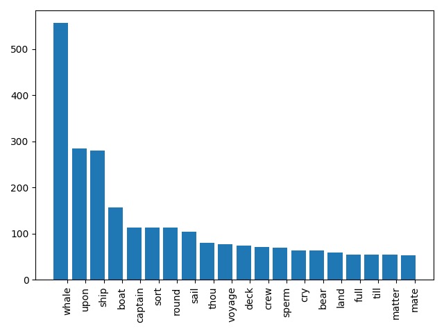
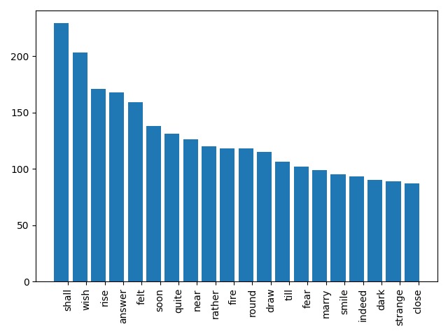
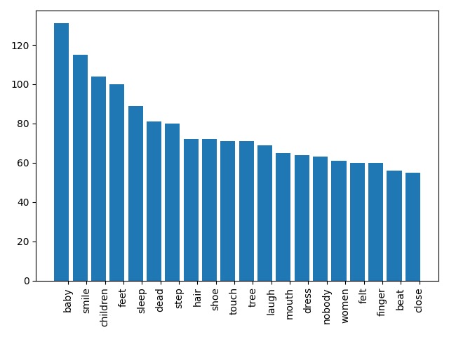
Figure 1: Three word frequency charts quickly generated by the DHLab. From left to right: Moby Dick, by Herman Melville; Jane Eyre, by Charlotte Brontë; and Beloved, by Toni Morrison.

In the digital humanities, as in all subjects, the first thing one should ask whenever faced with a new set of information is: so what? How can this lead us to an interesting conclusion or interpretation? When it comes to word counts, there are two options: we can take a large word count as evidence of the prevalence of a certain theme, or we can start looking at the distribution and the context of these common words. The former is okay, if somewhat underwhelming; the latter is ideal.

We examine word distributions using what we like to call “word progression” plots. These can help us see the shape of our word count data, which in turn offers us a sort of roadmap with which to navigate a given theme.

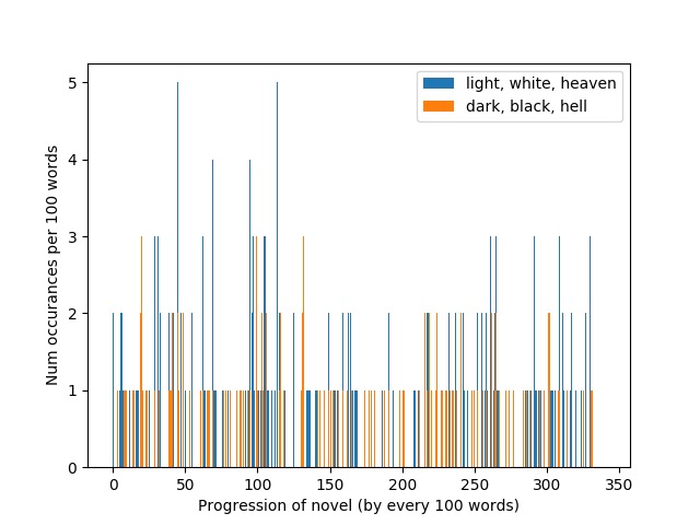
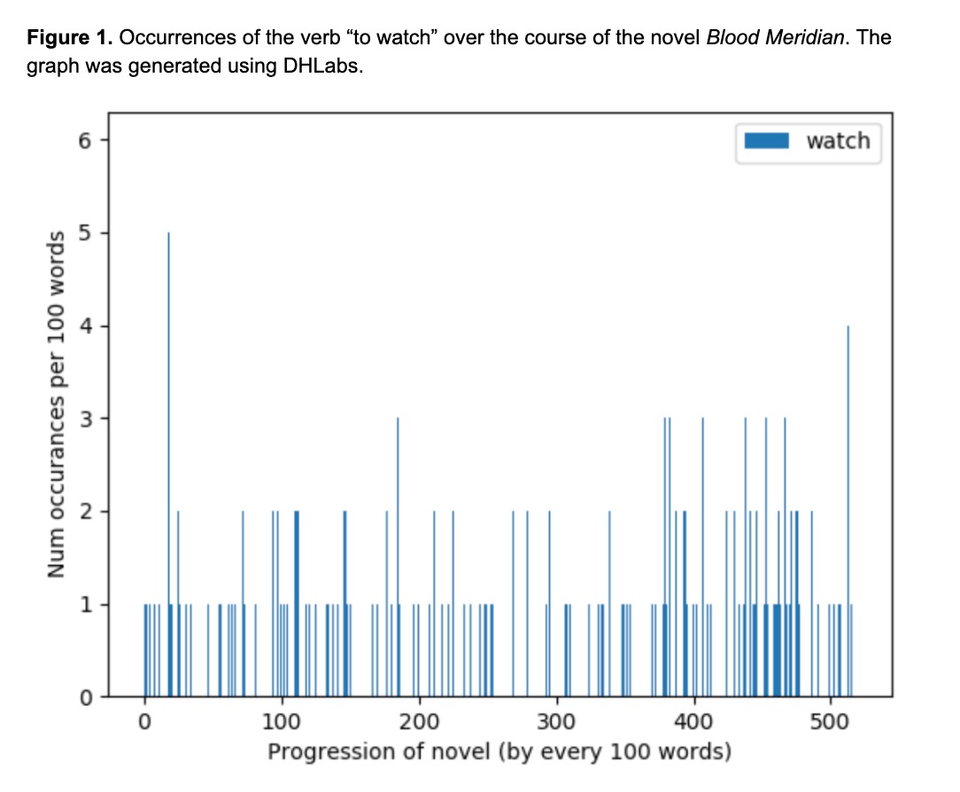
Figure 2: Examples of word progression plots for James Baldwin’s Go Tell it On the Mountain (left) and Cormac McCarthy’s Blood Meridian (right).

What kind of statements can these graphs support? Left: “The theme of darkness is spread rather evenly throughout the novel, while the theme of light shines through in specific moments with a forceful frequency.” Right: “Throughout his novel, McCarthy almost incessantly uses the verb ‘watching’ to note the observational role of various characters.

A tool that goes hand-in-hand with word progression plots is the passage sampling feature. This tool allows the reader to locate specific passages in which a word of interest shows up. This feature is very good at bringing the reader from the large-scale quantitative pattern perspective to the traditional deep-reading perspective of the English student. Think of it like a time machine that takes you on a guided tour across a story.

Oftentimes, word counts alone are not enough to justify the relevance of a given theme. For example, the word “nobody” seems to show up quite often in Morrison’s Beloved––but maybe it shows up just as often in other texts. There is a method by which to get a more powerful reading on word relevance, and it is called term frequency, inverse document frequency (tf-idf). tf-idf is a basic measure of how relevant a word is to a document relative to a whole corpus. It is rather intuitive––it takes into account the number of times a word shows up in a given text (“tf”) as well as how often it shows up in the greater corpus (“idf”). It is the product of tf and idf, which are calculated as follows.

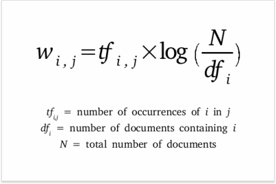
tf-idf opens the door to a new level of analysis. It gives us a more rigorous perspective on the word choice of certain authors. It allows us to think of texts as gigantic, easily comparable vectors, where each entry of the vector is the tf-idf of a word in the vocabulary. That would be very clunky to handle, of course, but it's a start (and vectorization of complex, ineffable things is what data science is all about, after all).

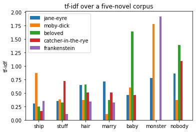
Figure 3: The tf-idf scores of various words in a corpus of three novels.

We can handpick certain words and certain texts and compare the relevance of certain words across them. See Figure 3 above. Different scores for words like “whale,” “marry,” and “woman” make sense in the context of the novels and serve as a sort of sanity check for the model. Meanwhile, score differences in words like “nobody” and “smile” are less obvious, and can lead to some interesting investigations.

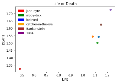
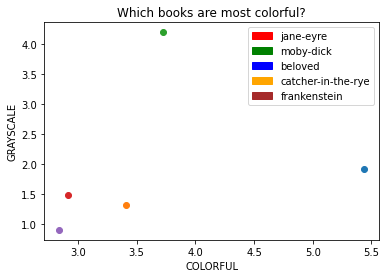
Figure 4: “Thematic vectorization” using tf-idf scores.

These are done by defining themes as lists of words, and then calculating the “relevance” of a theme to a given text by summing the tf-idf of all words in the theme. This allows us to plot novels in “theme space,” which opens us up to machine learning algorithms like k-means clustering.

The DHLab as it exists now is a lab in the sense that it enables numerical experimentation and analysis of text. However, as the project progresses, we envision a more literal manifestation of a lab, as in a research collective. We want the DHLab to help facilitate research projects and curricular initiatives; to become a sort of student consulting group for interdisciplinary research